I recently discovered the value of vlookup in excel. And I keeping finding more and more ways and reasons to use it. Last week a co-worker needed to compare values on a report from two different dates. We were chatting about it and I realized the vlookup would solve her problem.
In this example, I have sales reports from 3 separate days.
I want a quick look at how much revenue I made, by product, over all 3 days.
Step 1: I want a consolidated list of products.
- Step 1a: I’ll copy the values from column A in all 3 sheets into a new workbook
- Step 1b: I’ll highlight the column
- Step 1c: I’ll go to the Data Ribbon and select Remove duplicates
- Step 1d: When it asks me, I’ll confirm that I want to remove the duplicates
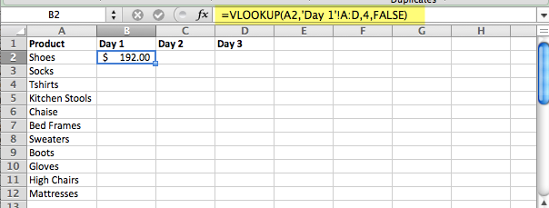
Step 2: Create Formula. =VLOOKUP(A2,’Day 1′!A:D,4,FALSE)
What this says is in English is:
- Go to sheet Day 1 [‘Day1’!],
- Look at the information in columns A thru D [A:D],
- Find the row that says “Shoes” [A2]
- Then give me the value that is in column 4 in the row that says “shoes”
- And only display information if the value in A2 is EXACTLY the same [FALSE].
The logic for the formula is in this order: the value we’re looking for [A2], the place where we are looking to find it [‘Day 1’!A:D], the column with the information we want to display [4], and we want exact values [FALSE]
Step 4: Use the formula for column C, but link to Day 2’s worksheet.
Step 5: Use the formula for Column C, but link to Day 3’s worksheet.
Step 6: Copy values down for all rows.
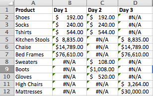
This is what you should end up with. Here’s the spreadsheet if you want to practice. You’ll notice that this returned errors for the products that didn’t sell on certain days. There are two solutions to this.
SOLUTION 1: more steps, but less complicated
If you won’t be constantly updating the spreadsheet, you can do a quick and easy copy/”paste value” and find/replace:
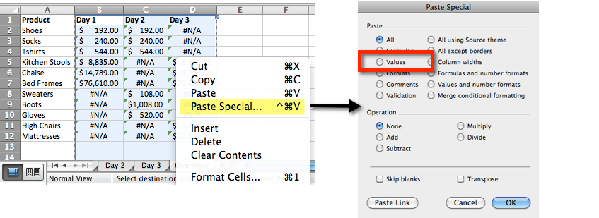
Step A: Select all cells
Step B: Copy. I prefer Command (or Control on PC) + C
Step C: Right click, select “Paste Special”, then select “Values”
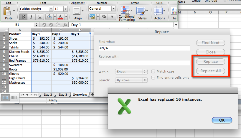
Step D: Do Find/Replace. I like to select Command (or Control for PC) + F, then select the “Replace” button. Type in #N/A in the Find box and leave the Replace box empty. Select “Replace All”
Now you have cleaned up data and you can run calculations or create charts with it.
SOLUTION 2: the more complicated formula solution
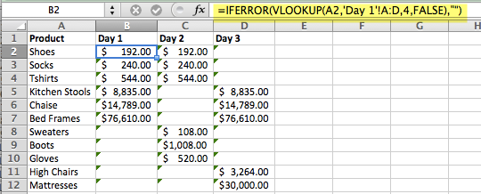
If you’ll be using this spreadsheet on an ongoing basis, I’d suggest an =IF( formula.
We’re starting with
=VLOOKUP(A2,’Day 1′!A:D,4,FALSE) and we’re going to change it to
=IFERROR(VLOOKUP(A2,’Day 1′!A:D,4,FALSE),””)
What this says in English is: If there’s an error when doing this formula, then give me a blank cell.



One response to “vlookup formula in Excel for Mac”
Great article… Here’s a video that is very helpful with the vlookup function