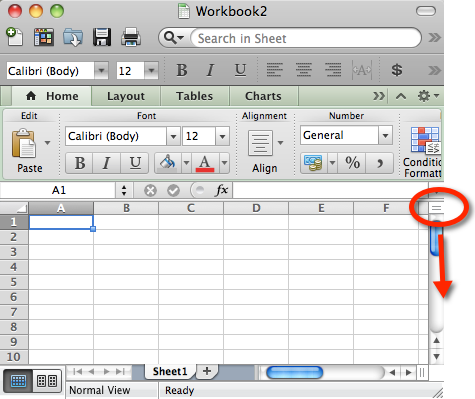
Step 1: Grab the bar on the far right side and drag down
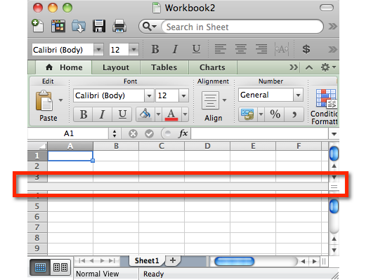
Step 2: Drag until the top bar to below the cells you want frozen at the top
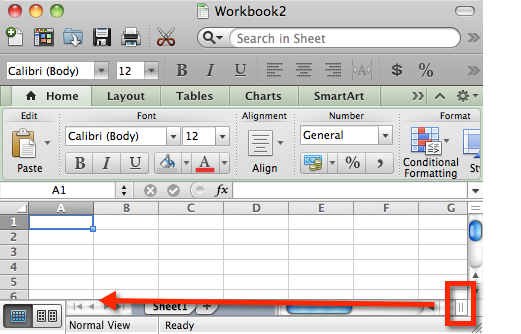
Step 3: Grab the bar on the bottom right and drag to the right.
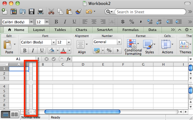
Step 4: Drag the bar until it is to the right of the cells you want frozen on the left.
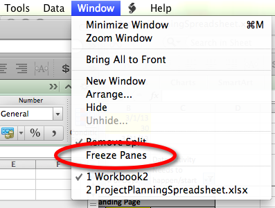
Step 5: Freeze the panes. On a Mac go to the Window menu and then select freeze pane. On a PC, you’ll go to the View menu. One nice time saver on the PC version is it has the option on the View / Freeze Pane menu to freeze the first row and/or the first column.
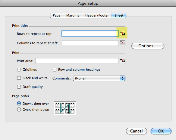
UPDATE: As a response to this post, my friend Michelle asked how to make the same rows print at the top of every page. Go to Page Set-up and select the “Sheet” tab. Click the strange button to the right of the “Rows to repeat at top:” box and then select the row(s) you want. The option to repeat columns on the left is right below if you want to do that.

17 responses to “How to Freeze Panes in Excel for Mac”
Actually, you can freeze panes without splitting the screen first. Just click on a cell then click on Window > Freeze panes. This will freeze the cells to the left of and above that cell. In the screen shown in your example, B4 would be the cell to click on first.
Thanks, Janice! I always appreciate tips to improve my Excel usage.
This comment was very helpful for Excel 08 on Lion, thank you!
Thanks! This was killing me today.
Thanks, Billy. I’m glad it was helpful!https://www.kristaveteto.com/wp-admin/edit-comments.php#comments-form
Krista, I’m definitely bookmarking this page. For some reason I just can’t keep it in my noggin how to do this. Your instructions are very clear and accurate. Thanks for your service to the computer-user world that we all co-habitat!
Awesome post! But what impressed me the most was your bio: “Jesus lover. Broken vessel. INFJ.” Way to keep it real!!
I have Excel 2008 for Mac. The option “freeze panel” seems to be realy an option i can’t use. Do i need an upgrade?
Oh… That was easy. Thanks!!!!
Thank you! This has been annoying me for days! Why it doesn’t work correctly when you simply select rows you want frozen, and then freeze panes… I have no idea.
you’re a star!
R
This not working for me. When I go to the Windows menu I see the Freeze Panes there but it is greyed out. 🙁
Were you able to figure out what was wrong? If not, what version of Excel are you using?
fantastic, i could not figure out how do freeze both first row and column and this helped heaps!! thanks!
Thanks – I’ve searched the web a bit and this is the first time I’ve seen something that actually works for the mac
Hi Your tip was useful for me, Thank u very much
So simply explained. Thank you. Wasted time on so many other websites
Thank you, Rick!